
1. Design Goals
When a stereo matching model is composed of “base model + auxiliary correction module”, joint training from the start runs into a fundamental training-order problem. The three-stage training plan is designed to solve precisely this problem.
1.1 Problem: the correction task is impossible
If the base model has never seen the target domain (e.g., the pretrained weights have never seen synthetic transparent-object data), training the correction module under such conditions produces:
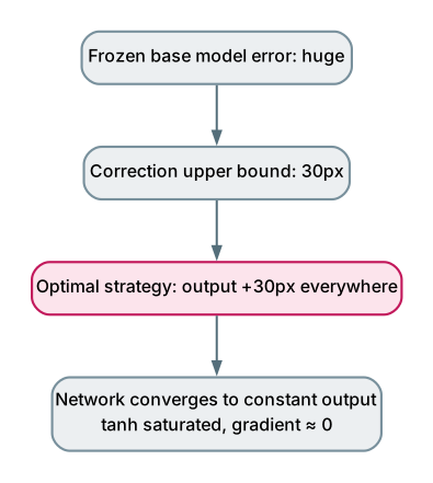
Root cause: the upper bound of the correction is far smaller than the base model’s error, so even a perfect correction can only fix a small portion. The network discovers that “always outputting the upper bound” is a local optimum; the saturated region of tanh has near-zero gradient and cannot learn spatial structure.
Core constraint: training the correction module while the base model has no understanding of the target domain makes the task itself impossible. The base model’s error must first be pushed below the correction’s upper bound before the correction task becomes feasible.
2. Architecture: Three-Stage Training Plan
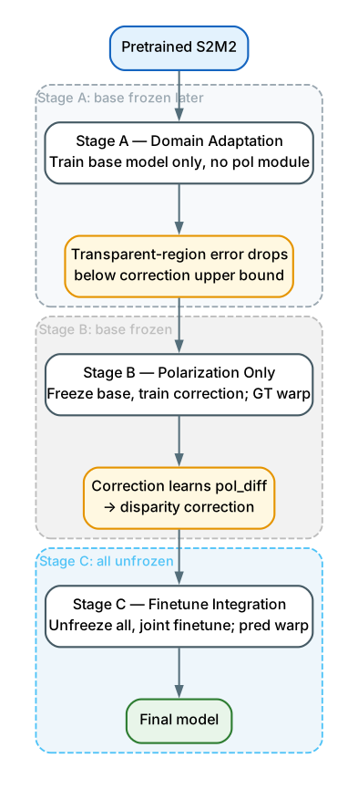
3. Three-Stage Components and Design
3.1 Stage A — Baseline Domain Adaptation
| Item | Setting |
|---|---|
| Goal | Let the base model first adapt to the target data domain |
| Input | Pretrained S2M2 weights |
| Training scope | Train only the base model; no polarization module |
| Expected effect | Error over transparent regions drops substantially below the correction’s upper bound |
| Key role | Establishes a reasonable foundation so the subsequent correction task becomes feasible |
3.2 Stage B — Polarization Only Learning
| Item | Setting |
|---|---|
| Goal | Let the correction module learn the pol_diff -> disparity correction mapping |
| Input | Stage A checkpoint |
| Training scope | Freeze the base model; train only the correction module |
| Warp mode | GT warp (ensures pol_diff quality) |
| Key role | base_err is already below max_correction, so the task is feasible |
Another reason to freeze the base model is to avoid a shortcut: if the base were trainable, it would take the shortcut of learning disparity directly, and the correction would not be forced to learn.
3.3 Stage C — Finetune Integration
| Item | Setting |
|---|---|
| Goal | Joint fine-tuning so the base and correction work together |
| Input | Stage B checkpoint |
| Training scope | Everything unfrozen; joint fine-tune |
| Warp mode | Switch to pred warp (simulates real inference) |
| Key role | Both modules are already pretrained, so joint tuning does not shortcut |
4. Why Three Stages Solve the Problem
| Problem | How the three-stage plan handles it |
|---|---|
| Base error too large; correction cannot move it | Stage A first pushes the base error below the correction’s upper bound |
| Correction does not learn (task impossible) | Stage B trains the correction under conditions where the task is feasible |
| Shortcut problem (base steals credit) | Stage B freezes the base, forcing the correction to learn from pol_diff |
| Joint training collapse | By Stage C both sides are pretrained, so joint tuning is stable |
The key feasibility constraint: before training, confirm max_correction >= base_error; otherwise the network cannot solve the task and will converge to a constant output. The role of Stage A is exactly to push base_error below max_correction.
5. Tensor / Training State Dimensions
| Stage | Trainable modules | Frozen modules | Source of warp disparity |
|---|---|---|---|
| Stage A | base model (S2M2) | — | not applicable (no polarization module) |
| Stage B | correction module | base model | GT disparity |
| Stage C | base model + correction module | — | predicted disparity |
6. Polarization Injection Points
The Pol injection point in the three-stage training enters the correction module via warp-based pol_diff. The three stages are a “training pipeline design”; they do not change the injection point itself, but progressively make the modules around the injection point reach a trainable state:
- Stage A: the correction module that hosts the injection point is not yet enabled.
- Stage B: the injection point is enabled; pol_diff is computed with GT warp; only the correction module is trained.
- Stage C: the injection point is enabled; pol_diff is computed with pred warp; the full model is jointly trained.
7. Design Decisions and Rationale
| Decision | Rationale |
|---|---|
| Add Stage A (Domain Adaptation) | Pretrained weights have not seen the target domain; base_error must first be pushed below max_correction |
| Freeze base model in Stage B | Avoids the base taking a shortcut and stealing credit; forces correction to learn from pol_diff |
| GT warp in Stage B | Ensures pol_diff quality so the correction learns semantics under perfect alignment |
| Unfreeze everything in Stage C joint fine-tune | Both modules are pretrained, so joint fine-tuning does not shortcut |
| Switch to pred warp in Stage C | Simulates the real inference setting |
| Three-stage as a general pattern | Domain Adaptation -> Module-specific Learning -> Joint Fine-tune applies to any “base + auxiliary module” architecture |
8. Highlights
- Breaks an impossible task through training order: first lower the base error, then train the correction, avoiding correction being forced to converge to a constant output when the base has no understanding of the domain.
- Explicit feasibility constraint: before training, use
max_correction >= base_erroras the task-feasibility criterion, and use tanh saturation (raw) as a danger signal. - Freezing the base prevents shortcut: Stage B freezes the base, forcing the correction to truly learn from pol_diff rather than letting the base shortcut and steal credit.
- Pretrain each side before joint fine-tuning: by Stage C both modules are in place, avoiding the situation where one side has not yet learned and is overwhelmed by the other.
- Transferable general training pattern: Domain Adaptation -> Module-specific Learning -> Joint Fine-tune applies to any two-stage “base + auxiliary module” architecture.