
1. Design Goals
Core problem: In real-world deployment there are only two cameras (left captures I∥, right captures I⊥), so it is impossible to obtain both polarization images from the same viewpoint. Therefore I∥ and I⊥ cannot be compared at the pixel level directly.
Design goal: Without same-viewpoint access to both polarizations, still embed polarization feedback into the stereo matching pipeline while keeping changes minimal — by reusing S2M2’s existing iterative refinement architecture as the injection point.
Key insights:
- Computing pol_diff does not require a perfect disparity; coarse alignment is enough.
- The quality of pol_diff improves as the disparity estimate improves.
- Polarization feedback can be embedded inside the existing refinement loop of S2M2, with no external two-stage pipeline required.
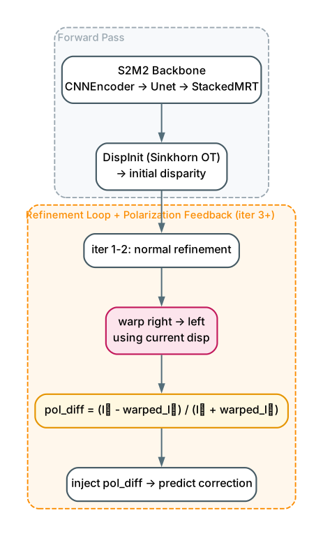
2. Architecture: Polarization-Aware Refinement
3. Components and Modules
3.1 S2M2PolarizationV2 (Base Version)
S2M2PolarizationV2 adds a Polarization refinement module on top of the original S2M2. The base version’s forward pass is:
class S2M2PolarizationV2(nn.Module):
    def __init__(self, base_model, pol_mode='normalized'):
        self.base_model = base_model  # Original S2M2
        self.pol_encoder = nn.Sequential(...)  # Processes pol_diff
        self.correction_net = nn.Sequential(...)  # Predicts disparity correction

    def forward(self, left, right):
        # 1. Base model forward
        disp, occ, conf = self.base_model(left, right)

        # 2. Warp right to left view
        warped_right = warp_right_to_left(right, disp)

        # 3. Compute polarization difference
        pol_diff = (left - warped_right) / (left + warped_right + eps)

        # 4. Predict and apply correction
        pol_feat = self.pol_encoder(pol_diff)
        correction = self.correction_net(cat([pol_feat, disp]))

        return disp + correction, occ, conf
3.2 warp-based pol_diff
Since both polarizations are not available from the same viewpoint, pol_diff is computed after warping the right image to the left view using disparity:
warped_right = warp_right_to_left(right, disp)
pol_diff = (I∥ - warped_I⊥) / (I∥ + warped_I⊥)
This is a normalized polarization difference, with eps added to the denominator to avoid division by zero. Coarse alignment suffices: as long as the initial disparity is roughly correct, pol_diff becomes meaningful.
4. Two-Stage Training Variant (GT/Pred warp)
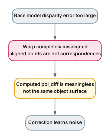
4.1 The Chicken-and-Egg Problem
warp-based pol_diff has a chicken-and-egg issue: a good disparity is needed to compute a good pol_diff, yet pol_diff is exactly what is supposed to improve the disparity. When the base model has large disparity errors over transparent regions:
4.2 Solution: Two-Stage Training
Core idea: first let the model learn the semantics of pol_diff under “perfect alignment”, then let it handle the case with alignment errors.
- Stage 1 (GT Warp): Use GT disparity for the warp. The correction module learns “what pol_diff means under correct alignment” and can focus on the pol_diff → disparity correction mapping.
- Stage 2 (Pred Warp): Use the predicted disparity for the warp. The model learns to work even when alignment is imperfect, similar to curriculum learning.
4.3 S2M2PolarizationV2 (Two-Stage Version) Code
class S2M2PolarizationV2(nn.Module):
    def __init__(self, ...):
        self.use_gt_warp = False  # Controlled by set_training_stage()

    def set_training_stage(self, stage: int):
        """stage=1: GT warp, stage=2: pred warp"""
        self.use_gt_warp = (stage == 1)

    def forward(self, left, right, gt_disp=None, return_diagnostics=False):
        disp, occ, conf = self.base_model(left, right)

        # Choose the disparity used for warping
        if self.use_gt_warp and gt_disp is not None:
            warp_disp = gt_disp  # Stage 1: perfect alignment
        else:
            warp_disp = disp     # Stage 2: use prediction

        # Warp and compute pol_diff
        warped_right = warp_right_to_left(right, warp_disp)
        pol_diff = compute_polarization_diff(left, warped_right)

        # Correction
        correction = self._predict_correction(pol_feat, disp)
        disp_refined = disp + correction

        if return_diagnostics:
            return disp_refined, occ, conf, {
                'base_disp': disp,
                'correction': correction,
                'pol_diff': pol_diff,
                'correction_scale': sigmoid(self.correction_scale) * 10,
            }
        return disp_refined, occ, conf
4.4 Training Strategy Notes
- Warmup: freeze the base model and train only the polarization components; then fine-tune everything together.
- Best-model selection: based on the error metric over transparent regions (lower is better).
- Validation always uses Stage 2 (pred warp) so that validation reflects the true inference setting.
4.5 Technical Notes
BCE Loss is incompatible with AMP:
# Wrong: BCE triggers an assertion failure under autocast
with autocast():
    loss = F.binary_cross_entropy(pred, target)

# Correct: BCE must be computed in float32
with autocast('cuda'):
    pred = model(x)
# Compute loss outside autocast
loss = F.binary_cross_entropy(pred.float(), target.float())
gt_conf must be clamped:
# Avoid NaN caused by extreme disparity errors
gt_conf = torch.exp(-disp_error.clamp(0, 100) / tau)
gt_conf = (gt_conf * valid_mask).clamp(0, 1)  # Ensure in [0, 1]
5. Correction Architecture Evolution
The correction module (correction_net) went through three revisions: original (triple suppression) → simplified → bounded.
5.1 Original: Triple Suppression
# Issues with the original architecture
self.correction_net = nn.Sequential(
    nn.Conv2d(65, 64, 3, padding=1),
    nn.GroupNorm(8, 64),      # <- GroupNorm suppresses spatial variation
    nn.ReLU(inplace=True),
    nn.Conv2d(64, 32, 3, padding=1),
    nn.GroupNorm(8, 32),      # <- Another GroupNorm
    nn.ReLU(inplace=True),
    nn.Conv2d(32, 1, 3, padding=1),  # <- zero init
)
nn.init.zeros_(self.correction_net[-1].weight)  # <- Suppression 1
nn.init.zeros_(self.correction_net[-1].bias)

correction = torch.tanh(x) * scale  # <- Suppression 2: tanh
scale = torch.sigmoid(self.correction_scale) * 10  # <- Suppression 3: sigmoid
Triple suppression:
- Zero init: output starts from 0.
- tanh: pulls large values back.
- sigmoid(scale): multiplies by a small number.
Problem: gradients must pass through all three layers before the correction can move, and the two GroupNorm layers further suppress spatial variation, causing the correction to output the same value for all pixels (std=0).
5.2 Simplified: Remove All Suppression
# Simplified: 2 conv layers, no suppression
self.correction_net = nn.Sequential(
    nn.Conv2d(1, 32, 3, padding=1),   # pol_diff -> 32ch
    nn.ReLU(inplace=True),
    nn.Conv2d(32, 1, 3, padding=1),   # 32ch -> correction
)
# No zero init, no tanh, no learnable scale
# Direct: correction = correction_net(pol_diff)
After simplification the correction regained spatial variation, but because ReLU outputs are unbounded, the correction values exploded toward ±∞. Removing “triple suppression” was overcorrected — output constraints were stripped away entirely.
5.3 Bounded: tanh × max_correction
# Fixed architecture (bounded version)
self.correction_net = nn.Sequential(
    nn.Conv2d(1, 32, 3, padding=1),
    nn.ReLU(inplace=True),
    nn.Conv2d(32, 1, 3, padding=1),
)
self.max_correction = 30.0  # Maximum correction magnitude (pixels)

# Forward
correction_raw = self.correction_net(pol_diff)
correction = torch.tanh(correction_raw) * self.max_correction  # Bounded in [-30, +30]
Keep tanh to constrain the output range, but drop zero init and the sigmoid scale.
5.4 Comparison of the Three Versions
| Property | Original (triple suppression) | Simplified (explodes) | Fixed (bounded) |
|---|---|---|---|
| Zero init | yes | no | no |
| tanh | yes | no | yes |
| sigmoid scale | yes | no | no |
| GroupNorm | yes (two layers) | no | no |
| Output range | 0 -> slowly grows | ±∞ | [-30, +30] |
| Issue | gradients cannot pass | explosion | balanced |
Why max_correction = 30: corrections should be learned progressively; large errors do not need to be fixed in a single step. 30 px is enough to make meaningful corrections without giving the network too much freedom.
5.5 Saturation Monitoring
Diagnose using correction_raw by tracking the pre-tanh mean absolute value:
corr: +5.23 (max:28.7, raw:1.45)
                       ^
              pre-tanh mean absolute value
Criteria:
raw < 1: learning normally, in the linear region of tanh.1 < raw < 2: approaching saturation, still trainable.raw > 3: severely saturated, gradients vanishing.
6. Tensor Dimensions
| Tensor | Shape / Description |
|---|---|
| left (I∥) / right (I⊥) | (B, 3, H, W) |
| disp / occ / conf | base model output |
| warped_right | (B, 3, H, W); right warped to left view using disp |
| pol_diff | (B, 1, H, W) or (B, C, H, W); normalized polarization difference |
| pol_feat | output of pol_encoder(pol_diff) |
| correction_net input (original) | 65 channels (pol_feat + disp concat) |
| correction_net input (simplified / bounded) | 1 channel (pol_diff) |
| correction_raw | (B, 1, H, W); pre-tanh |
| correction | (B, 1, H, W); bounded version constrained to [-30, +30] |
| disp_refined | disp + correction |
7. Polarization Injection Points
The Pol injection point of this module sits inside S2M2’s iterative refinement loop:
- iter 1-2: normal refinement, no polarization injected.
- iter 3+: polarization-aware refinement, with warp-based pol_diff injected.
- Injection flow: warp right -> left -> compute pol_diff -> pol_encoder -> correction_net predicts disparity correction ->
disp + correction.
This is a natural injection point that reuses S2M2’s existing iterative mechanism, with no external two-stage pipeline required.
8. Design Decisions and Rationale
| Decision | Rationale |
|---|---|
| warp-based pol_diff | Same-viewpoint polarization pairs are unavailable in the real world; alignment must be done via disparity warping |
| Embed into refinement loop (iter 3+) | Leverages S2M2’s existing iterative mechanism; minimal changes; no external pipeline |
| Two-stage training (GT -> Pred warp) | Resolves chicken-and-egg: first learn semantics under perfect alignment, then remove the training wheels |
| Validation fixed to Stage 2 | Validation must reflect true inference (pred warp) |
| Bounded correction with tanh × max_correction | Unbounded explodes; triple suppression suffocates; tanh × fixed scale is the balance point |
| max_correction = 30 | Enough for meaningful correction without giving the network excessive freedom |
| Remove GroupNorm | GroupNorm suppresses spatial variation; the correction map must retain spatial information |
| Compute BCE outside autocast | BCE is incompatible with AMP and must be computed in float32 |
9. Highlights
- Solves the unavailability of same-viewpoint polarization: by warping the right image to the left view via disparity, “only two cameras in real deployment” is no longer a barrier to polarization feedback.
- Embedded in the existing iterative mechanism: polarization feedback is injected at iter 3+ of S2M2’s existing refinement loop, with no external two-stage pipeline and minimal changes.
- Two-stage training breaks the chicken-and-egg: first learn pol_diff semantics under GT warp (perfect alignment), then switch to pred warp to adapt to alignment errors — similar to curriculum learning.
- Balance point for correction output constraints: triple suppression blocks gradients, no constraints explode; finally
tanh × max_correctionfinds the balance between “can learn” and “does not explode”. - Monitorable saturation: the pre-tanh mean absolute value of
correction_rawserves as a diagnostic indicator that immediately reveals whether tanh has entered saturation and gradients are vanishing.