
1. Design Goals
This architecture targets the matching difficulty over glass regions in active polarization stereo systems and adopts a “medium-capacity polarization path (Pol stream)” design. Its core idea:
Process the polarization signal with the same pyramid + lookup strategy as RGB
  - Keep the full 36ch polarization signal
  - No encoder/pooling
  - At every GRU iteration the model sees the complete profile at the current
    disparity
The design avoids two extremes: compressing the polarization signal with a 3D CNN + pooling washes out the peak at the correct disparity, while using only two statistics (max/var) is too sparse. The middle ground is to not compress and not pool — keep the full 36-channel polarization cost profile so that the α predictor sees the complete information at every GRU iteration.
2. Architecture
2.1 Initial Version
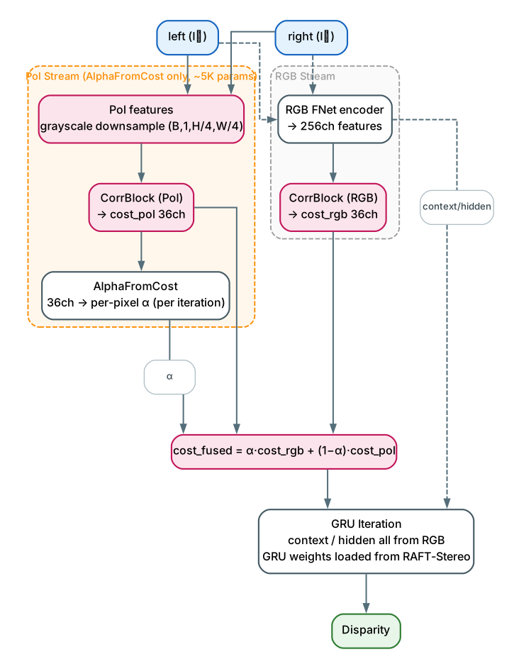
Key designs:
- α predicted at every iteration: from the 36-channel cost_pol at the current disparity.
- Sees the full profile: not compressed statistics.
- No encoder needed: grayscale images go directly into correlation.
2.2 Revised Version (CorrBlockNoNorm + Gaussian blur)
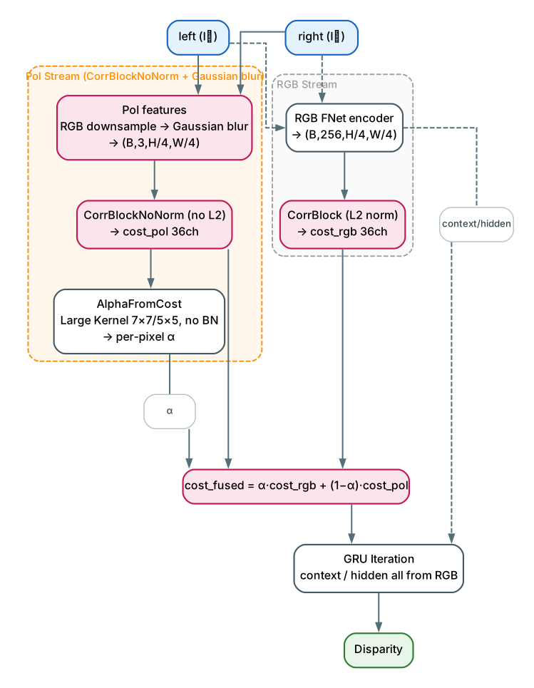
The revised version addresses two problems of the initial version: (1) the L2 normalization in the original CorrBlock kills the polarization intensity difference, so CorrBlockNoNorm is used instead; (2) once normalization is removed, high-frequency spurious signals appear in non-glass regions, so a Gaussian blur is added before correlation to suppress them.
3. Components and Modules
3.1 AlphaFromCost
Predicts per-pixel α from the 36-channel cost_pol at the current disparity of every GRU iteration.
class AlphaFromCost(nn.Module):
    """Predict per-pixel α from cost_pol (36ch)"""

    def __init__(self, corr_dim=36, hidden_dim=32):
        self.net = nn.Sequential(
            nn.Conv2d(corr_dim, hidden_dim, 3, padding=1),
            nn.ReLU(),
            nn.Conv2d(hidden_dim, hidden_dim, 3, padding=1),
            nn.ReLU(),
            nn.Conv2d(hidden_dim, 1, 1),
            nn.Sigmoid(),
        )
3.2 AlphaFromCost — Large Kernel Improved Version
To break the “BN dilemma” (BN ON washes out the polarization signal, BN OFF lets MC noise through), large kernels are used: large kernels naturally smooth high-frequency noise while preserving region-level polarization patterns, removing the need for BN.
class AlphaFromCost(nn.Module):
    def __init__(self, corr_dim=36, hidden_dim=32):
        self.net = nn.Sequential(
            # 7x7 kernel: region-level judgment
            nn.Conv2d(corr_dim, hidden_dim, kernel_size=7, padding=3),
            nn.ReLU(),
            # 5x5 kernel
            nn.Conv2d(hidden_dim, hidden_dim, kernel_size=5, padding=2),
            nn.ReLU(),
            # 1x1 output
            nn.Conv2d(hidden_dim, 1, kernel_size=1),
            nn.Sigmoid(),
        )
Design rationale:
- MC noise averages out within the 7×7 receptive field.
- The region-level structure of the polarization signal is preserved.
- No BN needed (avoids washing out the magnitude difference).
3.3 CorrBlockNoNorm
The original CorrBlock applies L2 normalization before computing correlation. L2 normalization eliminates the “intensity difference” (after normalization, I∥ and I⊥ become almost identical), and the essence of the polarization signal is exactly this intensity difference. Hence a CorrBlock without normalization is designed for the Pol stream.
Original CorrBlock:
class CorrBlock:
    def _build_corr(self, fmap1, fmap2):
        # L2 Normalization
        fmap1 = fmap1 / (torch.norm(fmap1, dim=1, keepdim=True) + 1e-6)
        fmap2 = fmap2 / (torch.norm(fmap2, dim=1, keepdim=True) + 1e-6)

        corr = torch.einsum('bchw,bchx->bhwx', fmap1, fmap2)  # dot product
        return corr
CorrBlockNoNorm:
class CorrBlockNoNorm:
    """No L2 normalization; preserves polarization intensity difference"""

    def _build_corr(self, fmap1, fmap2):
        # No normalization! compute dot product directly
        corr = torch.einsum('bchw,bchx->bhwx', fmap1, fmap2)
        return corr
3.4 Gaussian Blur (Low-pass Filter)
Once normalization is removed, non-glass regions develop high-frequency spurious signals (MC noise + texture noise). Adding a Gaussian blur before correlation suppresses the high-frequency noise while preserving the low-frequency polarization structure.
def _get_pol_features(self, left, right):
    # Downsample
    left_feat = F.interpolate(left, size=(h, w), ...)
    right_feat = F.interpolate(right, size=(h, w), ...)

    # Low-pass filter (Gaussian blur)
    left_feat = gaussian_blur(left_feat, kernel_size=5)
    right_feat = gaussian_blur(right_feat, kernel_size=5)

    return left_feat, right_feat
Why blur before correlation: what needs to be eliminated is the high-frequency noise in the input images; smoothing first and then computing correlation is cleaner than computing correlation first and smoothing afterwards.
4. Tensor Dimensions
| Item | Dimensions | Description |
|---|---|---|
| Pol features (initial) | (B, 1, H/4, W/4) | Grayscale downsampling |
| Pol features (revised) | (B, 3, H/4, W/4) | RGB downsampling + Gaussian blur |
| cost_pol | (B, 36, H/4, W/4) | CorrBlockNoNorm pyramid + lookup |
| RGB features | (B, 256, H/4, W/4) | fnet encoder output |
| cost_rgb | (B, 36, H/4, W/4) | CorrBlock (with L2 norm) pyramid + lookup |
| AlphaFromCost input | (B, 36, H/4, W/4) | cost_pol |
| α | (B, 1, H/4, W/4) | Per-pixel fusion weight |
| cost_fused | (B, 36, H/4, W/4) | α-weighted fusion |
5. Hyperparameters
| Parameter | Default | Description |
|---|---|---|
| corr_dim | 36 | Number of cost_pol channels (AlphaFromCost input) |
| hidden_dim | 32 | AlphaFromCost hidden channel count |
| Gaussian blur kernel | 5 | Low-pass filter size used before correlation |
| Large Kernel sizes | 7×7 / 5×5 | Kernel sizes of the improved AlphaFromCost |
| Pol parameter count | ~5K | Total parameters of AlphaFromCost |
6. Design Decisions and Rationale
6.1 Same Pyramid + Lookup as RGB
Pyramid + lookup preserves the full 36-channel polarization signal so that every GRU iteration sees the complete cost profile at the current disparity. The α predictor needs to see the complete disparity profile to correctly distinguish glass from non-glass.
6.2 L2 Normalization Removed
L2 normalization is fine for learned features (256ch), but for raw pixels (3ch) it kills the polarization signal (eliminates intensity differences). Correlation measures similarity rather than difference; polarization makes I∥ ≠ I⊥ on glass, so removing the normalization leaves at least some variation to work with.
6.3 Gaussian Blur Separates Signal from Noise
Polarization is region-level structure; noise is pixel-level randomness. Gaussian blur smooths high-frequency noise while preserving low-frequency structure.
6.4 Large Kernels Break the BN Dilemma
BN is a double-edged sword:
| BN State | Polarization Signal | MC Noise |
|---|---|---|
| ON | Washed out | Suppressed |
| OFF | Preserved | Let through |
Characteristic differences between MC noise and the polarization signal:
| Characteristic | MC Noise | Polarization Signal |
|---|---|---|
| Spatial frequency | High frequency (pixel-level random) | Low frequency (region-level structure) |
| Spatial correlation | None (i.i.d.) | Strong (continuous over glass regions) |
| Physical source | Monte Carlo sampling error | Polarized specular reflection |
Large kernels distinguish signal from noise via spatial structure rather than via statistical normalization, so they preserve the polarization signal while suppressing MC noise without needing BN.
7. Highlights
- Full 36-channel polarization profile: processes the polarization signal with the same pyramid + lookup strategy as RGB; no compression, no pooling — every GRU iteration sees the complete cost profile at the current disparity.
- Iteration-level α prediction: AlphaFromCost predicts per-pixel α at each GRU iteration from the 36-channel cost_pol at the current disparity, rather than relying on one-shot static statistics.
- CorrBlockNoNorm preserves polarization intensity: a custom CorrBlock without L2 normalization for the polarization path, avoiding the elimination of the “intensity difference” on which the polarization signal depends.
- Gaussian blur separates signal from noise: a low-pass filter before correlation suppresses pixel-level high-frequency noise while preserving the region-level low-frequency polarization structure.
- Large kernels replace BN: 7×7 / 5×5 large kernels distinguish signal from noise via “spatial structure”, resolving the dilemma of “BN ON washes out the signal, BN OFF lets the noise through” without any normalization.