1. Design Goals
This architecture targets the matching difficulty over glass regions in active polarization stereo systems and adopts an “ultra-lightweight polarization path (Pol stream)” design: while keeping the dual-stream structure, the learnable parameters on the polarization side are reduced to the absolute minimum.
1.1 Core Insight: Pol’s Job Is Actually Simple
Pol only needs to tell the model "where the glass is":
  - Glass region:    |I∥ - I⊥| large -> α should be small (don't trust RGB)
  - Non-glass region: |I∥ - I⊥| ≈ 0 -> α should be large (trust RGB)

This only needs a simple detector, not a full stereo matching pipeline!
The core of the polarization signal is the brightness difference |I∥ - I⊥|, which is a simple physical quantity. Deciding “where is the glass” is essentially a binary classification problem and does not need a full feature extractor or context encoder. This architecture builds on that insight by drastically simplifying the Pol stream, keeping only a tiny α predictor.
2. Architecture
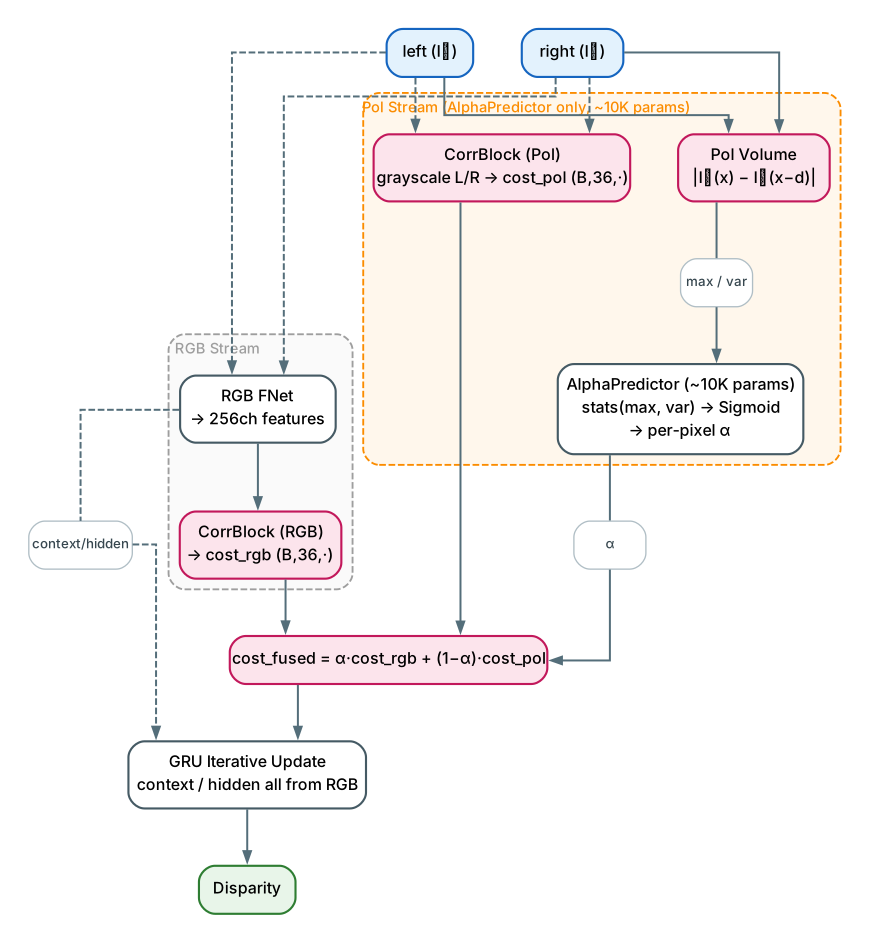
Design highlights:
- The Pol stream keeps only a tiny AlphaPredictor and has no learned feature extractor or context encoder.
- Context and hidden states come entirely from the RGB stream.
- The only learnable Pol component is the tiny AlphaPredictor.
3. Components and Modules
3.1 AlphaPredictor (max/var Statistics)
The core of this architecture. It does not encode the Pol Volume in a learned way; instead, it first takes two statistics (max, var) along the disparity axis via “deterministic computation”, then uses a tiny 2–3 layer conv network to map these statistics into per-pixel α.
class AlphaPredictor(nn.Module):
    """
    Predict per-pixel α from statistics of the Pol Cost Volume

    Input: Pol Cost Volume (B, D, H, W)
    Statistics:
      - max along disparity axis: peak polarization difference
      - var along disparity axis: degree of variation
    Output: α (B, 1, H, W)

    Parameter count: ~10K
    """
    def __init__(self, hidden_dim=16):
        self.net = nn.Sequential(
            nn.Conv2d(2, hidden_dim, 3, padding=1),
            nn.ReLU(),
            nn.Conv2d(hidden_dim, hidden_dim, 3, padding=1),
            nn.ReLU(),
            nn.Conv2d(hidden_dim, 1, 1),
            nn.Sigmoid(),
        )

    def forward(self, pol_volume):
        pol_max = pol_volume.max(dim=1, keepdim=True)[0]
        pol_var = pol_volume.var(dim=1, keepdim=True)
        stats = torch.cat([pol_max, pol_var], dim=1)
        return self.net(stats)
pol_max: the maximum polarization difference along the disparity axis, corresponding to “glass has a peak at the correct d”.pol_var: the degree of variation along the disparity axis.- The two are concatenated into a 2-channel input for the conv network, then passed through Sigmoid to output α in [0, 1].
3.2 Cost Fusion
Pol and RGB use the same pyramid + lookup strategy, both yielding 36 channels, then fused by α-weighting.
# RGB: 256-dim features -> correlation -> pyramid -> lookup -> 36 channels
corr_block_rgb = CorrBlock(fmap_rgb_left, fmap_rgb_right)
cost_rgb = corr_block_rgb(disp)  # (B, 36, H/8, W/8)

# Pol: grayscale -> correlation -> pyramid -> lookup -> 36 channels
fmap_pol_left = left.mean(dim=1, keepdim=True)  # grayscale
fmap_pol_right = right.mean(dim=1, keepdim=True)
corr_block_pol = CorrBlock(fmap_pol_left, fmap_pol_right)
cost_pol = corr_block_pol(disp)  # (B, 36, H/8, W/8)

# Fusion
cost_fused = alpha * cost_rgb + (1 - alpha) * cost_pol
4. Tensor Dimensions
| Item | Dimensions | Description |
|---|---|---|
| Pol Volume | (B, D, H, W) | Raw ` |
| pol_max | (B, 1, H, W) | max along disparity axis |
| pol_var | (B, 1, H, W) | var along disparity axis |
| AlphaPredictor input | (B, 2, H, W) | concat(pol_max, pol_var) |
| α | (B, 1, H, W) | Per-pixel fusion weight |
| cost_rgb | (B, 36, H/8, W/8) | RGB correlation pyramid + lookup |
| cost_pol | (B, 36, H/8, W/8) | Grayscale correlation pyramid + lookup |
| cost_fused | (B, 36, H/8, W/8) | α-weighted fusion |
5. Hyperparameters
| Parameter | Default | Description |
|---|---|---|
| hidden_dim | 16 | AlphaPredictor hidden channel count |
| Pol parameter count | ~10K | Total parameters of AlphaPredictor |
6. Design Decisions and Rationale
6.1 Replace Learned Encoding with Statistics
The core of the polarization signal is the brightness difference |I∥ - I⊥|, a simple physical quantity. Statistics (max, var) capture it effectively, without learning a complex feature extractor.
6.2 α Is a “Glass Detector”, Not a “Feature Fuser”
The essence of α is telling the model “is this glass?”, a binary classification problem that does not need a complex network. The AlphaPredictor only needs to learn the mapping “max/var → glass/non-glass”.
6.3 Single-Stage Training
- AlphaPredictor has only ~10K parameters.
- The statistics (max, var) are deterministic computations, with nothing to learn.
- AlphaPredictor only needs to learn the “max/var → glass/non-glass” mapping.
- This mapping is simple and can be trained jointly with the GRU in a single stage, without stage-wise training.
6.4 Design Complexity Should Match Problem Complexity
When the problem is intrinsically simple (glass detection), use a simple solution. The ultra-lightweight Pol stream is exactly about matching design complexity to problem complexity.
7. Highlights
- Ultra-lightweight Pol stream: the learnable parameters on the polarization side are compressed to about 10K — just a 2–3 layer conv AlphaPredictor, with no learned feature extractor or context encoder at all.
- Deterministic statistical input: max (peak polarization difference) and var (degree of variation) are extracted along the disparity axis via deterministic computation; the AlphaPredictor only needs to learn the simple mapping “statistics → glass probability”.
- Single-stage training: since there is no large network on the polarization side to learn from scratch, the α predictor can be trained jointly with the GRU in a single stage, keeping the pipeline simple.
- Context/Hidden fully reused from RGB: the polarization side is responsible only for producing α-weighting and does not participate in context or hidden states, maximally reusing the existing RGB path.
- Design complexity matches problem complexity: treats “glass detection” as a binary classification problem and pairs it with the smallest possible network, avoiding over-design.