
1. Design Goals
When the polarization residual is injected into the correlation volume, even if an iteration schedule controls “when to inject pol”, the question of “where to inject pol” remains unsolved — regardless of region, the residual strength only depends on the iteration.
But the locations where polarization should intervene are spatially varying: regions with large gradients in the disparity map are often object boundaries, occlusions, or matching-hard regions — exactly where stereo is less reliable and pol should step in.
The design goal of this architecture is: use the disparity gradient as an uncertainty proxy, giving pol more say in “uncertain regions”. On top of the iteration schedule, multiply in a spatial gate driven by the disparity gradient.
2. Architecture Mechanism: Gradient Gating
disp_grad = compute_gradient(disp).detach()  # stop-grad to avoid feedback loop!
gate = GatingNetwork(pol_corr, disp_grad)    # tiny network, sigmoid → [0, 1]
alpha = i / max(iters - 1, 1)                # iteration schedule
corr_enhanced = corr + alpha * gate * pol_residual(pol_corr)
The overall formula is a three-way multiplicative modulation: corr + α · gate · residual.
α(iteration schedule):i / max(iters-1, 1), controls “when” to inject pol.gate(gradient gating): produced byGatingNetwork, controls “where” to inject pol.residual: polarization residual produced byPolCorrResidual, controls the injected content.
3. Design Points
3.1 disp_grad.detach() — stop-gradient
disp_grad = compute_gradient(disp).detach()
disp_gradis the spatial gradient of the current disparity estimate, serving as a structural cue for “uncertainty”..detach()blocks gradient backpropagation: avoids forming a feedback loop.- Without detach, the network could take a shortcut of “manipulating disparity to make the gate larger/smaller” to minimize loss, degrading the gate into a learnable shortcut and losing its physical meaning.
- After detach,
disp_gradis purely a side signal that “reads the shape of disparity” — it is a structural cue rather than a learnable shortcut.
3.2 GatingNetwork is tiny
GatingNetwork is deliberately designed to be very small:
- Only 2 conv layers.
- No BatchNorm.
- No attention.
- Inputs are
pol_corranddisp_grad; sigmoid at the end outputs a gate in [0, 1].
Design rationale: this is a mechanism proof, not a black box. The smaller the network, the more we can confirm that “gradient gating as a mechanism” itself is effective, rather than being brute-fit by the capacity of a large network.
3.3 α × gate
- Using gate alone has a problem: in early iterations the disparity is still coarse,
disp_gradis itself noisy, and the gate is unreliable. - Therefore the iteration schedule
alphais kept:α × gateensures that even if the gate is noisy in early iterations, the overall injection strength is still suppressed by α≈0. - Only in mid/late iterations, after disparity stabilizes, does
disp_gradbecome meaningful and the gate truly take effect.
4. Architecture (Data Flow)
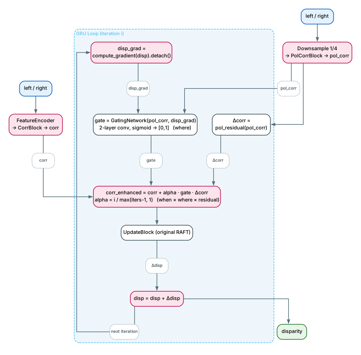
5. Components and Modules
5.1 GatingNetwork
Takes pol_corr and the detached disp_grad as input, passes through 2 conv layers (no BN, no attention), and ends with sigmoid to output a spatial gate of shape (B, 1, H, W) with values in [0, 1].
5.2 PolCorrResidual
Three convolutional layers (3×3 → 3×3 → 1×1) plus a learnable scalar scale, with the last layer initialized to 0, outputting a polarization residual Δcorr projected to corr_dim.
5.3 Schedule Coefficient alpha
alpha = i / max(iters - 1, 1), a fixed function of iteration, not a learnable parameter.
6. Tensor Dimensions
| Tensor | Shape / Type | Description |
|---|---|---|
disp | (B, 1, H, W) | Current disparity estimate |
disp_grad | (B, *, H, W) | Spatial gradient of disparity, detached |
pol_corr | (B, pol_dim, H, W) | Output of PolCorrBlock |
gate | (B, 1, H, W) | Output of GatingNetwork, in [0, 1] |
alpha | scalar | Iteration schedule |
Δcorr | (B, corr_dim, H, W) | Output of pol_residual |
corr_enhanced | (B, corr_dim, H, W) | corr + α·gate·Δcorr |
7. Hyperparameters
| Hyperparameter | Value | Description |
|---|---|---|
pol_levels | 4 | Number of pyramid levels in the polarization volume |
pol_radius | 4 | Lookup radius of the polarization volume |
iters | 24 | Number of GRU iterations (also determines the length of the α schedule) |
8. Design Decisions and Rationale
| Decision | Rationale |
|---|---|
| Use disparity gradient as uncertainty proxy | High-gradient regions (boundaries/occlusions) are mostly stereo-unreliable regions, exactly where pol should step in |
disp_grad.detach() | Blocks the feedback loop, prevents the gate from degrading into a learnable shortcut |
GatingNetwork is only 2 conv layers, no BN, no attention | Mechanism proof — validates the mechanism itself rather than relying on network capacity |
Keep the iteration schedule alpha and multiply with the gate | Early-iteration disp_grad is noise; suppressed by α≈0 |
| Residual and UpdateBlock follow the standard design | Adds a “where” dimension on top of “when”; everything else unchanged |
9. Highlights
- Uses the disparity gradient as an uncertainty proxy, letting the polarization residual automatically focus on object boundaries, occlusions, and other stereo-unreliable regions.
- The injection formula
corr + α · gate · residualis a three-way multiplicative modulation — α controls “when”, gate controls “where”, and residual controls the “content”. disp_grad.detach()blocks gradient backpropagation, preventing the network from manipulating disparity to turn the gate into a learnable shortcut, so gradient gating retains its physical meaning.GatingNetworkis deliberately tiny (2 conv layers, no BN, no attention), positioned as mechanism validation to ensure that the effect comes from the gating mechanism itself rather than from network capacity.- The
α × gatemultiplicative design elegantly handles the early-iteration disparity noise: even if the gate is unreliable, overall injection is still suppressed by α≈0.